Perceptron
Like the brain neuron, it is bi-stated.
fires when input summation going above threshold value
Given input-output pairs, can make itself learn through changing weights.
Used as a building block in Different brand of current NNs even though not used now
Learning of Perceptron
- Random initialization of weights
- Patterns are applied one by one.
- Positively misclassified input, weights decreased in proportion with the input
- Negatively misclassified inputs, weights are decreased by the same proportion.
- When all patterns are over, the whole set is reapplied until no wrong answer is got.
- For a linearly separable problem, Perceptron can always solve the problem, Perceptron Convergence theorem of Rosenblatt says.
- The learning of Perceptron is analogous to adjusting water tap containing cold and hot water inputs
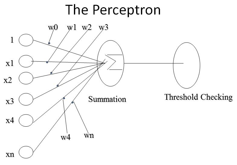
How Perceptron computes
- Let Input is a vector (x1,x2,..xn)
- x0 = 1 (to have the effect of threshold)
- g(x) = S n i=0 (wi * xi) for i=0 to n
- o(x) = 0 if g (x) < 0 else 1
- If two inputs then g(x) = w0+w1x1+w2x2
- When g(x) is 0, w2 = -(w1/w2)*x1- w0/w2
- This is an equation of decision surface
- Sign of g(x) determines whether Perceptron fires or not, while magnitude ( the value of g(x)) determines how far it is from the decision surface.
- Let w be the set of weights (w0,w1,...wn)
- let X be the subset of training instances misclassified by the current set of weights
- J(w) is the Perceptron Criterion function
- J(w) = S(S(wi*xi)for i=0 to n) for all x belongs to X
- J(w) = E(|wx|) for all x belongs to X
- J(w) = E w * x if x is misclassified as a negative example otherwise w*-x if x is misclassified as a positive example.
- Let d(J) = S(x) where x is taken positive if x misclassified as a negative example, otherwise x is taken negative.
- dis called a gradient which is telling us the direction in which we should move to reduce J, i. e. the direction of solution
- New set of weights is determined as follows
- w(t+1) = w(t) + h * d(J)
Perceptron Learning Algorithm
- Given a Classification problem with n input features and 2 output classes
- The solution sought is the one out of potentially infinite number of weight vectors that will cause the Perceptron to fire whenever the input falls into the first output class
- n+1 inputs and n+1 weights are taken, where x0 always set to 1
- All weights are initialized to different random values.
- Iterate through The training set, collecting all inputs misclassified by the current set of weights.
- If all inputs are classified correctly, output the weights and quit.
- Otherwise compute the vector sum S of the misclassified input vectors, where each vector has the form (x0,x1,..xn). In Creating the sum add S to vector x if x is an input for which the Perceptron incorrectly fails to fire, but add -x if x is an input for which Perceptron incorrectly fires. Multiply the sum by scale factor h
- Modify the weights (w0..wn) by adding the elements of the vector S to them. Go to Iteration step.
Analysis of the algorithm :-
- It is a search process of its kind. It starts from a state where all weights are random and stops when get the weights which constitutes the solution
- The decision surface is a line here. There can be infinite equations of a line so infinite no. of weight vectors possible to get. This is also true for other cases
Problem with Perceptron learning algorithm
- Answer can’t be sought when no decision surface exists. i.e for EXOR problem.
- Multilayer Perceptrons can solve problem by creating multiple decision surfaces.
- But it was not known how to train middle layer weights. With fixed handcoded weights , though problem could be solved.
- Perceptron Convergence theorem could not be extended to Multilayer networks
Multilayer Perceptrons and Backpropagation
- Backpropagation is a systematic method of training multilayer Perceptrons
- It was first shown by Werbos in 1974, then Parker doing the same in 1982 and the same is rediscovered by Rumelhart and others in 1986.
- Despite of limitations Backpropagation has dramatically expanded the range of problems which could be solved thru NN
- Backpropagation uses an algorithm which has strong mathematical background.
- It requires an activation function which is everywhere differentiable.
- It is using a sigmoid type Activation function compared to a squared Activation function by single layer Perceptron.
- Sigmoid allows automatic gain control and also it is useful in bettering a trained weight.
Comparison of Activation Functions
Multi-layer Perceptron
Multilayer network
- Multilayer Network Shown earlier is trained by Backpropagation algorithm.
- First layer is known as input, Second is known as hidden and the third is known as output layer.
- The first layer just distributes the inputs, other layers sums and applies the sigmoid function to their respective inputs.
- There are two layers of weights.
- There is inconsistency in literature about the layers in the Network.